![]()
If you don't want to print now,
Statistical inference
The term statistical inference describes statistical techniques that obtain information about a population parameter (or parameters) based on a single random sample from that population. There are two different but related types of question about the population parameter (or parameters) that we might ask:
What parameter values would be consistent with the sample data?
This branch of inference is called estimation and its main tool is a confidence interval. We described confidence intervals in the previous chapter.
A manufacturer of muesli bars needs to describe the average fat content of the bars (the mean of the hypothetical population of fat contents that would be produced using the recipe). Several bars are analysed and their fat contents are measured.
The sample mean is a point estimate of the population mean, and a 95% confidence interval can also be found.
Are the sample data consistent with some statement about the parameters?
This branch of inference is called hypothesis testing and is the focus of this chapter.
A particular brand of meusli bar is claimed by the manufacturer to have a fat content of 3.4g per bar. A consumer group suspects that the manufacturer is understating the fat content, so a random sample of bars is analysed.
The consumer group must assess whether the data are consistent with the statement (hypothesis) that the underlying population mean is 3.4g.
Errors and strength of evidence
When we studied parameter estimation, we saw that a population parameter cannot be determined exactly from a single random sample — there is a 5% chance that a 95% confidence interval will not include the true population parameter.
In a similar way, a single random sample can rarely provide enough information about a population parameter to allow us to be sure whether or not any hypothesis about that parameter will be true. The best we can hope for is an indication of the strength of the evidence against the hypothesis.
The remainder of this chapter explains how this evidence is obtained and reported.
Randomness in sports results
Although we like to think that the 'best' team wins in sports competitions, there is actually considerable variability in the results. Much of this variability can be considered to be random — if the same teams play again, the results are often different. The most obvious examples of this randomness occur when a series of matches is played between the same two teams.
Since the teams are virtually unchanged in any series, the variability in results can only be explained through randomness.
Randomness or skill?
When we look at sports results, can we tell whether all teams are equally matched with the same probability of winning? Or do some teams have a higher probability of winning than others?
There are different ways to examine this question, depending on the type of data that is available. The following example assesses an end-of-year league table.
English Premier Soccer League, 2008/09
In the English Premier Soccer league, each of the 20 teams plays every other team twice (home and away) during the season. Three points are awarded for a win and one point for a draw. The table below shows the wins, draws, losses and total points for all teams at the end of the 2008/09 season.
Team |
Wins | Draws | Losses | Points | |
|---|---|---|---|---|---|
| 1. 2. 3. 4. 5. 6. 7. 8. 9. 10. 11. 12. 13. 14. 15. 16. 17. 18. 19. 20. |
Manchester_U Liverpool Chelsea Arsenal Everton Aston_Villa Fulham Tottenham West_Ham Manchester_C Wigan Stoke_City Bolton Portsmouth Blackburn Sunderland Hull_City Newcastle Middlesbrough West_Brom_Albion |
28 25 25 20 17 17 14 14 14 15 12 12 11 10 10 9 8 7 7 8 |
6 11 8 12 12 11 11 9 9 5 9 9 8 11 11 9 11 13 11 8 |
4 2 5 6 9 10 13 15 15 18 17 17 19 17 17 20 19 18 20 22 |
90 86 83 72 63 62 53 51 51 50 45 45 41 41 41 36 35 34 32 32 |
We observed in an earlier simulation that there is considerable variability in the points, even when all teams are evenly matched. However, ...
If some teams are more likely to win their matches than others, the spread of final points is likely to be greater — the top and bottom teams are likely to be more extreme.
A simulation
To assess whether there is any difference in skill levels, we can therefore run a simulation of the league, assuming evenly matched teams and generating random results with probabilities 0.372, 0.372 and 0.255 for wins, losses and draws. (A proportion 0.255 of games in the actual league resulted in draws.)
Click Simulate to simulate the 380 games in a season. The standard deviation of the final points is shown below the table. Click Accumulate then run the simulation about 100 times. (Hold down the Simulate button to speed up the process.)
The standard deviation of the points in the actual league table was 18.2. Since most simulated standard deviations are between 5 and 12, we conclude that such a high spread would be extremely unlikely if the teams were evenly matched.
There is strong evidence that the top teams are 'better' than the bottom teams.
Other uses of simulation
Simulations can help us to answer questions about a variety of other models (or populations). The following example shows another simple simulation.
Is security at LA International Airport as good as elsewhere?
In 1987, the Federal Aviation Administration (FAA) investigated security at Los Angeles International Airport (LAX). In one test, it was found that only 72 out of 100 mock weapons that FAA inspectors tried to carry onto planes were detected by security guards (Gainesbille Sun, Dec 11, 1987).
Is the FAA justified in claiming that this "detection rate was well below the national rate of 0.80"?
A simulation
If the detection rate at LAX was the same as elsewhere, and every weapon independently has probability 0.80 of being detected, we know that the number detected out of 100 weapons will be a random quantity.
How unlikely is it to get as few as 72 out of 100 weapons detected if the probability of detection at LAX is 0.80 — the same as elsewhere?
A simulation helps to answer this question.
Click Simulate to randomly 'try to get 100 weapons onto planes', with each independently having probability 0.80 of detection. Click Accumulate then run the simulation between 100 and 200 times. (Hold down the Simulate button to speed up the process.)
Observe the distribution of the number of weapons detected. The proportion of simulations with 72 or fewer weapons being detected is shown to the right of the dot plot. Observe that this rarely happens.
We therefore conclude that the FAA's claim that LAX has a poorer detection rate than elsewhere is justified — only 72 weapons being detected would be unlikely if the detection rate was really 0.80.
We will return to this example later.
Assessing a claim about a mean
In this example, we ask whether a sample mean is consistent with the underlying population mean having a target value.
Quality control for cornflake packets
In a factory producing packets of cornflakes, the weight of cornflakes that a filling machine places in each packet varies from packet to packet. From extensive previous monitoring of the operation of the machine, it is known that the net weight of '500 gm' packets is approximately normal with standard deviation σ = 10 gm.
The mean net weight of cornflakes in the packets is controlled by a single knob. The target is for a mean of µ = 520 gm to ensure that few packets will contain less than 500 gm. Samples are regularly taken to assess whether the machine needs to be adjusted. A sample of 10 packets was weighed and contained an average of 529 gm. Does this indicate that the underlying mean has drifted from µ = 520 and that the machine needs to be adjusted?
A simulation
If the filling machine is working to specifications, each packet would contain a weight that is sampled from a normal distribution with µ = 520 and σ = 10.
How unlikely is it to get the mean of a sample of size 10 that is as far from 520 as 529 if the machine is working correctly?
A simulation helps to answer this question.
Click Simulate to randomly generate the weights of 10 packets from a normal (µ = 520, σ = 10) distribution. Click Accumulate then run the simulation between 100 and 200 times. (Hold down the Simulate button to speed up the process.)
Observe that although many of the individual cornflake packets weigh more than 529 gm, it is rare for the mean weight to be as far from the target as 529 gm (i.e. either ≥529 gm or ≤511 gm).
There is therefore strong evidence that the machine is no longer filling packets with a mean weight of 520 gm and needs adjusting — a sample mean of 529 gm would be unlikely if the machine was filling packets to specifications.
We will return to this example later.
Simulation and randomisation
Simulation and randomisation are closely related techniques. Both are based on assumptions about the model underlying the data and involve randomly generated data sets.
Randomisation is understood most easily through an example.
Comparing two groups
If random samples are taken from two populations, we are often interested in whether the populations have the same means.
If the two populations were identical, any allocation of the sample values to the two groups would have been as likely as the observed sample data. By observing the distribution of the difference in means from such randomised allocations of values to groups, we can get an idea of whether the actual difference in sample means is unusually large.
An example helps to explain this method.
Characteristics of failed companies
A study in Greece compared characteristics of 68 healthy companies with those of another 33 that had recently failed. The jittered dot plots on the left below show the ratio of current assets to current liabilities for each of the 101 companies.
The mean asset-to-liabilities ratio for the sample of failed companies is 0.902 lower than that for the healthy companies, but the distributions overlap. Might this difference be simply a result of randomness, or can we conclude that there is a difference in the underlying populations?
Click Randomise to randomly pick 33 of the the 101 values for the failed group. If the underlying distribution of asset-to-liabilities ratios was the same for healthy and failed companies, each such randomised allocation would be as likely as the observed data.
Click Accumulate and repeat the randomisation several more times. Observe that the difference in means would rarely be as far from zero as -0.902 when we assume the same distribution for both groups. This strongly suggests that the distributions must be different.
Since the actual difference is so unusually large, ...
We can conclude that there is strong evidence that the mean asset-to-liability ratio is lower for failed companies than healthy ones.
In this page, another example of randomisation is described to assess whether teams in a soccer league are evenly matched.
English Premier Soccer League, 2007/08 and 2008/09
We saw earlier that the distribution of points in the 2008/09 English Premier Soccer League Table was not consistent with all teams being evenly matched — the spread of points was too high. We will now investigate this further.
If some teams are better than others, the positions of teams in the league in successive years will tend to be similar. The table below shows the points for the teams in two seasons. (Note that the bottom three teams are relegated each year and three teams are promoted from the lower league, so we cannot compare the positions of six of the teams.)
| Points | ||
|---|---|---|
|
Team |
2007/08 | 2008/09 |
| ManchesterU Chelsea Arsenal Liverpool Everton AstonVilla Blackburn Portsmouth ManchesterC WestHam Tottenham Newcastle Middlesbro Wigan Sunderland Bolton Fulham Reading Birmingham DerbyCounty StokeCity HullCity WestBromA |
87 85 83 76 65 60 58 57 55 49 46 43 42 40 39 37 36 36 35 11 - - - |
90 83 72 86 63 62 41 41 50 51 51 34 32 45 36 41 53 - - - 45 35 32 |
Manchester United, Chelsea, Arsenal and Liverpool were the top four teams in both years. However, ...
| Excluding Manchester United, Chelsea, Arsenal and Liverpool, do there seem to be any differences in ability between the other teams? |
Randomisation
If all other teams have equal probabilities of winning against any opponent, the 2008/09 points of 45 (which was actually obtained by Wigan) would have been equally likely to have been obtained by any of the teams in that year. Indeed, any allocation of the points (63, 62, 41, ..., 53) to the teams (Everton, Aston Villa, Blackburn, ..., Fulham) would be equally likely.
The diagram below performs this randomisation of the results in 2008/09.
Click Randomise to shuffle the 2008/09 points between the teams (excluding the top four teams and those that were only in the league for one of the seasons). If the teams were of equal ability, these points would have been as likely as the actual ones.
The correlation coefficient between the points in the two seasons gives an indication of how closely they are related. Click Accumulate and repeat the randomisation several more times. Observe that the correlation for the randomised values is only as far from zero as the actual correlation (r = 0.537) in about 5% of randomisations. Since a correlation as high as 0.537 is fairly unusual for equally-matched teams, ...
There is moderately strong evidence of a difference in skill between teams, even when the top four have been excluded.
A general framework
The examples in earlier pages of this section involved different types of data and different analyses. Indeed, you may find it difficult to spot their common theme!
All analyses were examples of hypothesis testing. We now describe the general framework of hypothesis testing within which all of these examples fit. This general framework is the basis for important applications in later sections of CAST.
The concepts in this page are extremely important — make sure that you understand them well before moving on.
Data, model and question
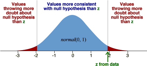
Either the null hypothesis or the alternative hypothesis must be true.
Approach
We assess whether the null hypothesis is true by asking ...
Are the data consistent with the null hypothesis?
It is extremely important that you understand that hypothesis testing addresses this question — make sure that you remember it well!!
Answering the question
| p-value | Interpretation |
|---|---|
| over 0.1 | no evidence that the null hypothesis does not hold |
| between 0.05 and 0.1 | very weak evidence that the null hypothesis does not hold |
| between 0.01 and 0.05 | moderately strong evidence that the null hypothesis does not hold |
| under 0.01 | strong evidence that the null hypothesis does not hold |
Use the pop-up menu below to check how the earlier examples in this section fit into the hypothesis testing framework.
Soccer league in one season
Inference and random samples
The examples in the previous section involved a range of different types of model for the observed data. In the remainder of this chapter, we concentrate on one particular type of model — random sampling from a population.
We assume now that the observed data are a random sample from some population.
When the observed data are a random sample, inference asks questions about characteristics of the underlying population distribution — unknown population parameters.
For random samples, the null and alternative hypotheses specify values for the unknown population parameters.
Inference about categorical populations
When the population distribution is categorical, the unknowns are the population probabilities for the different categories. To simplify, we consider populations for which one category is of particular interest ('success') and we denote the unknown probability of success by π.
The null and alternative hypotheses are therefore specified in terms of π.
Weapon detection at LAX
FAA agents tried to carry 100 weapons onto planes at LA International Airport. Of these, 72 were detected by security guards, and we are interested in whether this is consistent with the national probability of detection, 0.80.
We model detection of weapons as a random sample of 100 categorical values from a population with probability π of success (detection). The null hypothesis of interest is therefore...
H0: π = 0.80
The alternative hypothesis is
HA: π < 0.80
Telepathy experiment
An experiment is conducted to investigate whether one subject can telepathically pass shape information to another subject. A deck of cards containing equal numbers of cards with circles, squares and crosses is shuffled. One subject selects cards at random and attempts to 'send' the shape on the card to the other subject who is seated behind a screen; this second subject reports the shape imagined for the card. From 90 cards, the second subject correctly identifies 36.
This situation can be modelled as random sampling of 90 values (correct or wrong) from a categorical population in which the probability of correctly identifying the card is π. The null hypothesis of interest is therefore...
H0: π = 1/3 (guessing)
The alternative hypothesis is
HA: π > 1/3 (telepathy)
Tests about parameters of other populations
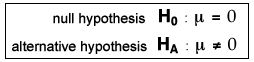
Other data sets arise as random samples from different kinds of population. For example, numerical data sets are often modelled as random samples from a normal distribution. Again, the hypotheses of interest are usually expressed in terms of the parameters of this distribution.
For example, to test whether the mean of a normal distribution is zero, the hypotheses would be...
H0: µ = 0
HA: µ ≠ 0
In the remainder of this section, we show how to test a population probability, and in the next section we will describe tests about a population mean.
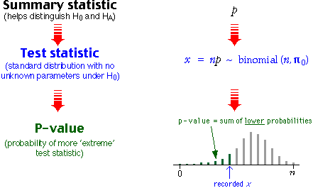
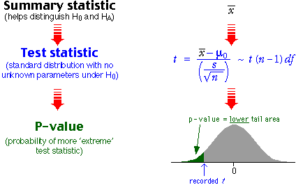
Test statistic
When testing the value of a probability, π, the obvious statistic to use from our random sample is the corresponding sample proportion, p.
It is however more convenient to use the number of successes, x, rather than p since we know that X has a binomial distribution with parameters n (the sample size) and π.
![]()
When we know the distribution of the test statistic (at least after the null hypothesis has fixed the value of the parameters of interest), it becomes much easier to obtain the p-value for the test.
P-value
As in all other tests, the p-value is the probability of getting such an 'extreme' set of data if the null hypothesis is true. Depending on the null and alternative hypotheses, the p-value is therefore the probability that X is as big (or sometimes as small) as the recorded value.
Since we know the binomial distribution of X when the null hypothesis holds, the p-value can therefore be obtained by adding binomial probabilities.
The p-value is a sum of binomial probabilities
Note that the p-value can be obtained exactly without need for simulations or randomisation.
Weapon detection at LAX
FAA agents tried to carry 100 weapons onto planes at LA International Airport, and 72 of these were detected by security guards. Is this consistent with the national probability of detection, 0.80?
H0: π = 0.80
HA: π < 0.80
In the diagram below, click Accumulate then hold down Simulate until about 100 samples of 100 values have been generated. The proportion of these simulated samples in which 72 or fewer weapons are detected is an approximation to the p-value for the test.
Since we know that the number detected has a binomial (100, 0.80) distribution when the null hypothesis holds, the simulation is unnecessary. Select Binomial distribution from the pop-up menu. This binomial distribution is displayed, and the probability of 72 or fewer detected weapons is shown to be 0.0342 — the p-value for the test.
Since the p-value is so small, there would have been very little chance of the observed data arising if LAX had probability 0.80 of detection. We can therefore conclude that there is strong evidence that the probability of detection is lower than this. Note that this can be done without any simulations.
Another example
The following example shows again how the binomial distribution can be used to obtain the p-value for a test about a population probability.
Telepathy experiment
In the telepathy experiment that was described at the start of this section, one subject selects cards with a random shape (circle, square or cross) and attempts to 'send' this shape to another subject who is seated behind a screen; this second subject reports the shape imagined for the card.
Out of 90 cards, 36 are correctly guessed. Since more than a third are correct, does this provide strong evidence that information is being telepathically transmitted?
The null and alternative hypotheses are...
H0: π = 1/3 (guessing)
HA: π > 1/3 (telepathy)
The p-value is the probability of getting 36 or more cards correct when π = 1/3. This can be obtained directly from a binomial distribution with π = 1/3 and n = 90.
Use the slider below to obtain the p-value for this test.
The p-value for the test is 0.1103, meaning that there is a probability of 0.1103 of getting 36 or more correct cards if there is no telepathy. We therefore conclude that there is no evidence of telepathy from the data.
Interpretation of p-values
If the p-value for a test is very small, the data are 'inconsistent' with the null hypothesis. (The observed data may still be possible, but are at least extremely unlikely.)
From a very small p-value, we can conclude that the null hypothesis is probably wrong.
However a high p-value cannot allow us to conclude that the null hypothesis is correct — only that the observed data are consistent with it. For example, if exactly 30 cards (a third) were correctly picked in the telepathy example above, it would be wrong to conclude that there was no telepathy. The data are also consistent with other values of π near 1/3, so we cannot conclude that π is not 0.32 or 0.34.
A hypothesis test can never conclude that the null hypothesis is correct.
The correct interpretation of p-values for the telepathy test would be...
| p-value | Interpretation | Conclusion |
|---|---|---|
| p > 0.1 | x is not unusually high. It would be as high in more than 10% of samples if π = 1/3. | There is no evidence against π = 1/3. |
| 0.05 < p < 0.1 | We would find x as high in only 5% to 10% of samples if π = 1/3. | There is only slight evidence against π = 1/3. |
| 0.01 < p < 0.5 | We would find x this high in only 1% to 5% of samples if π = 1/3. | There is moderately strong evidence against π = 1/3. |
| p < 0.01 | We would find x this high in under 1% of samples if π = 1/3. | There is strong evidence against π = 1/3. |
Finding the p-value for a one-tailed test
The LAX weapon-detection hypothesis test involved a random sample of size n from a population with probability π of success (detection of weapon). The data collected were x successes, and we tested the hypotheses...
![]()
where π0 was the constant of interest (e.g. 0.96 in this example). The following steps were followed to obtain the p-value for the test.
The diagram below illustrates these steps
The telepathy example was similar, but the alternative hypothesis involved high values of π and the p-value was found by counting upper tail probabilities.
Finding the p-value for a two-tailed test
The appropriate tail probability to use depends on the alternative hypothesis. If the alternative hypothesis allows either high or low values of x, the test is called a two-tailed test,
![]()
The p-value is then double the smaller tail probability since values of x in both tails of the binomial distribution would provide evidence for HA.
Somali blood groups
In a study of sab bondsmen, a population sub-group in Northern Somalia, blood tests were conducted on a sample of 54, in order to investigate whether they differed genetically from the main population of 'free-born noble Somali'.
It is known that a proportion 0.574 of free-born noble Somali have blood group O. (Actually 574 had blood group O in a sample of 1000, but this sample size was large enough to provide a reasonably accurate estimate.) Is there any evidence that the sample proportion with blood group O in the sab bondsmen, 26 out of 54, does not come from a population with π = 0.574? This can be expressed as the hypotheses
![]()
We would expect (0.574 × 54) = 31 of the sab bondsmen to have blood group O. A sample count that is either much greater than 31 or much less than 31 would suggest a genetic difference between the sab bondsmen and the free-born noble Somali. Use the slider below to obtain the p-value.
The probability of getting as few as 26 is 0.1084. Since this is a 2-tailed test, we must also take account of the probability of getting a count that is as unusually high, so the p-value is twice this, 0.2169. Getting 26 sab bondsmen with blood group O is therefore not unlikely, so we conclude that there is no evidence from these data of a genetic difference between sab bondsmen and the free-born Somali.
Computational problem
To find the p-value for a hypothesis test about a proportion, tail probabilities for a binomial distribution must be summed.
If the sample size n is large, there may be a huge number of probabilities to add together and this is both tedious and may result in numerical errors.
Home-based businesses owned by women
A recent study that was reported in the Wall Street Journal sampled 899 home-based businesses and found that 369 were owned by women.
Are home-based businesses less likely to be owned by females than by males? This question can be expressed as a hypothesis test. If the population proportion of home-based businesses owned by females is denoted by π, the hypotheses can be written as...
![]()
If the null hypothesis is true, the sample number owned by females will have a binomial distribution with parameters n = 899 and π = 0.5. The p-value for the test is therefore the sum of binomial probabilities,
![]()
A lot of probabilities must be evaluated and summed! And all are close to zero.
Normal approximation
We saw earlier that the normal distribution may be used as an approximation to the binomial when n is large. Both the sample proportion of successes, p, and the number of successes, x = np, are approximately normal when n is large.
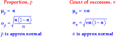
The best-fitting normal distribution can be used to obtain an approximation to any binomial tail probability. In particular, it can be used to find an approximate p-value for a hypothesis test.
Approximate p-value
A large random sample of size n is selected from a population with probability π of success and x successes are observed. We will again test the hypotheses
![]()
The normal approximation to the distribution of x can be used to find the tail probability,
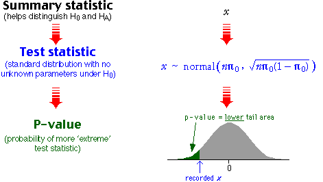
Home-based businesses owned by women
In this example, the sample size, n = 899 is large, so we can use a normal approximation to obtain the probability of 369 or fewer businesses owned by females if the underlying population probability was 0.5 (the null hypothesis).
Click Accumulate then simulate sampling of 899 businesses about 300 times. (Hold down the button Simulate.) From the simulation, it is clear that the probability of obtaining 369 or fewer businesses owned by females is extremely small — there is strong evidence against the null hypothesis.
The same conclusion can be reached without a simulation.
Select Bar chart from the pop-up menu, then select Normal approximation. From the normal approximation, we can determine that the p-value for the test (the tail area below 369) is extremely close to zero.
Continuity correction (advanced)
The approximate p-value could be found by comparing the z-score for x,
![]()
with a standard normal distribution. Since x is discrete,
P(X ≤ 369) = P(X ≤ 369.5) = P(X ≤ 369.9) = ...
To find this tail probability, any value of x between 369 and 370 might have been used when evaluating the z-score. The p-value can be more accurately estimate by using 369.5. This is called a continuity correction.
The continuity correction involves either adding or subtracting 0.5 from the observed count, x, before finding the z-score.
Be careful about whether to add or subtract — the probability statement should be unchanged. For example, P(X ≥ 410) = P(X ≥ 409.5), so 0.5 should be subtracted from x = 410 as a continuity correction in order to find this probability using a normal approximation and z-score.
The continuity correction is most important when the observed count is near either 0 or n.
Difference between parameter and estimate
Many hypothesis tests are about a single parameter of the model:
It is natural to base a test about such a parameter on the corresponding sample statistic:
If the value of the sample statistic is close to the hypothesised value of the parameter, there is no reason to doubt the null hypothesis. However if they are far apart, the data are not consistent with the null hypothesis and we should conclude that the alternative hypothesis holds.
A large distance between the estimate and hypothesized value is evidence against the null hypothesis.
Statistical distance
How do we tell what is a large distance between, say, p and a hypothesised value for the population proportion, π0? The empirical rule says that we expect p to be within two standard errors of π0 (about 95% of the time). If we measure the distance in standard errors, we know that 2 (standard errors) is a large distance, 3 is a very large distance, and 1 is not much.
The number of standard errors is
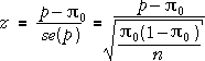
In general, the statistical distance of an estimate to a hypothesised value of the underlying parameter is
![]()
If this comes to more than 2, or less than -2, it suggests that the hypothesized value is wrong: the estimate is not consistent with the hypothesised parameter value. If, on the other hand, z is close to zero, the data are giving a result reasonably close to what we expected based on the hypothesis.
Test statistic and p-value
The statistical distance of an estimate to a hypothesised value of the underlying parameter is
![]()
This can be used at test statistic. If the null hypothesis holds, it approximately has a standard normal distribution — a normal distribution with zero mean and unit standard deviation.
The p-value for a test can be determined from the tail areas of this standard normal distribution.
In the above diagram, the null hypothesis is consistent with with estimates close to the hypothesised value and the alternative hypothesis is suggested by estimates that are either much bigger or smaller than this value (called a two-tailed test). For a two-tailed test, the p-value is the red tail area and can be looked up using either normal tables or in Excel.
Refinements
If the standard error of the estimate must itself be estimated from the sample data, the above test statistic is only approximately normally distributed. In some tests that we will describe in later sections, the test statistic has a t distribution (which has slightly longer tails than the standard normal distribution). This refinement will be described fully in the next section.
Home-based businesses owned by women
The diagram below repeats the simulation that we used earlier to test whether the proportion of home-based businesses owned by women was less than 0.5:
![]()
The proportion owned by women in a sample of n = 899 businesses was 369/899 = 0.410.
Again click Accumulate and hold down the Simulate button until about 100 samples of 899 businesses have been generated with a population probability of being owned by women of 0.5.
Select Statistical distance from 0.5 from the top pop-up menu to translate the proportions of female owners in the simulated samples into z-scores. Observe that most of these 'statistical distances from 0.5' are between -1 and +1.
The observed proportion owned by females was 0.410, corresponding to a statistical distance of z = -5.37, an unlikely value if the population proportion was 0.5.
Select Normal distribution from the lower pop-up menu to show the theoretical distribution of the z-scores. The p-value for the test is the tail area of this normal(0, 1) distribution below -5.37 and is virtually zero, so we again conclude that:
It is almost certain that π is less than 0.5.
Relation to previous test
The p-value obtained in this way using a 'statistical distance' as the test statistic is identical to the p-value that was found from a normal approximation to the number of successes without a continuity correction. (The p-value is slightly different if a continuity correction is used.)
The use of 'statistical distances' does not add anything when testing a sample proportion, but it is a general method that will be used to obtain test statistics in many other situations later in this e-book.
Tests about numerical populations
The most important characteristic of a numerical population is usually its mean, µ. Hypothesis tests therefore usually question the value of this parameter.
Blood pressure of executives
The medical director of a large company looks at the medical records of 72
male executives aged between 35 and 44 and observes that their mean blood pressure
is ![]() = 126.07.
We model these 72 blood pressures as a random sample from an underlying population
with mean µ
(blood pressures of similar executives) .
= 126.07.
We model these 72 blood pressures as a random sample from an underlying population
with mean µ
(blood pressures of similar executives) .
Published national health statistics report that in the general population for males aged 35-44, blood pressures have mean 128 and standard deviation 15. Do the executives conform to this population? Focusing on the mean of the blood pressure distribution, this can be expressed as the hypotheses,
![]()
Active ingredient in medicine
Pharmaceutical companies routinely test their products to ensure that the amount of active ingredient is within tight limits. However the chemical analysis is not precise and repeated measurements of this same specimen differ slightly. One type of analysis has errors that are normally distributed with mean 0 and standard deviation 0.0068 grams per litre.
A product is tested three times with the following concentrations of the active ingredient:
0.8403, 0.8363 and 0.8447 grams per litre
Are the data consistent with the target concentration of 0.86 grams per litre? This can be expressed as a hypothesis test comparing...
![]()
Null and alternative hypotheses
Both of the above examples involve tests of hypotheses
![]()
where µ0 is the constant that we think may be the true mean. These are called two-tailed tests. In other situations, the alternative hypothesis may involve only high (or low) values of µ (one-tailed tests), such as
![]()
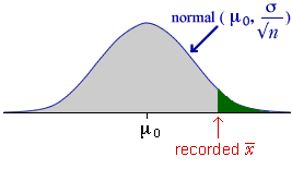
Model and hypotheses
In both examples in the first page of this section, there was knowledge of the population standard deviation σ (at least when H0 was true). This greatly simplifies the problem of finding a p-value for the test.
In both examples, the hypotheses were of the form,
![]()
Summary Statistic
The first step in finding a p-value for the test is to identify a summary statistic
that throws light on whether H0 or HA is true.
When testing the population mean, µ,
the obvious summary statistic is the sample mean, ![]() ,
and the hypothesis tests that will be described here are based on this.
,
and the hypothesis tests that will be described here are based on this.
We saw earlier that sample mean has a distribution with mean and standard deviation
![]()
![]()
Furthermore, the Central Limit Theorem states that the distribution of the sample mean is approximately normal, provided the sample size is not small. (The result holds even for small samples if the population distribution is also normal.)
P-value
The p-value for the test is the probability of getting a sample mean as 'extreme' as the one that was recorded when H0 is true. It can be found directly from the distribution of the sample mean.
Note that we can assume knowledge of both µ and σ in this calculation — the values of both are fixed by H0
Since we know the distribution of the sample mean (when H0 is true), the p-value can be evaluated as the tail area of this distribution.
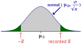
Statistical distance and test statistic
The p-value for testing a hypothesis about the mean, µ, when σ is known, is a tail area from the normal distribution of the sample mean and can be evaluated in the usual way using a z-score. This calculation can be expressed in terms of the statistical distance between the parameter and its estimate,
![]()
In the context of a test about means,
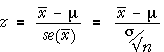
Since z has a standard normal distribution (zero mean and unit standard deviation) when the null hypothesis holds, it can be used as a test statistic.
P-value
The p-value for the test can be determined from the tail areas of the standard normal distribution.
For a two-tailed test, the p-value is the red tail area.
Quality control for cornflake packets
The diagram below repeats the simulation that we used earlier to test whether a sample mean weight of 10 cornflake packets of 529 gm is consistent with a packing machine that is set to give normally distributed weights with µ = 520 gm and σ = 10 gm.
Again click Accumulate and hold down the Simulate button until about 100 samples of 10 packets have been selected and weighed. The p-value is the probability of getting a sample mean further from 520 gm than 529 gm — either below 511 gm or above 529 gm and the simulation provides an estimate. However a simulation is unnecessary since we can evaluate the p-value exactly.
Select Normal distribution from the pop-up menu on the bottom right to replace the simulation with the normal distribution of the mean,
![]()
![]()
From its tail area, we can calculate (without a simulation) that the probability of getting a sample mean as far from 520 as 529 is exactly 0.0044. This is the exact p-value for the test.
P-value from statistical distance
Finally, consider the statistical distance of our estimate of µ, 529 gm, from the hypothesised value, 520 gm.

Select 'Statistical distance' from 520 from the middle pop-up menu to show how the p-value is found using this z-score.
Since the p-value is so small (0.0044), we conclude that there is strong evidence that the population mean, µ, is not 520.
Weights of courier packages
A courier company suspected that the weight of recently shipped packages had dropped. From past records, the mean weight of packages was 18.3 kg and their standard deviation was 7.1 kg. These figures were based on a very large number of packages and can be treated as exact.
Thirty packages were sampled from the previous week and their mean weight was found to be 16.8 kg. The data are displayed in the jittered dot plot below.
If the null hypothesis was true, the sample mean would have the normal distribution shown in pale blue. Although the sample mean weight is lower than 18.3 kg, it is not particularly unusual for this distribution, so we conclude that there is no evidence that the mean weight has reduced.
The right of the diagram shows how the p-value is calculated from a statistical distance (z-score).
Choose Modified Data from the pop-up menu. The slider allows you to investigate how low the sample mean must become in order to give strong evidence that µ is less than 18.3.
Unknown standard deviation
In the examples on the previous page, the population standard deviation, σ, was a known value. Unfortunately this is rarely the case in practice, so the previous test cannot be used.
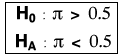
Saturated fat content of cooking oil
Both cholesterol and saturated fats are often avoided by people who are trying to lose weight or reduce their blood cholesterol level. Cooking oil made from soybeans has little cholesterol and has been claimed to have only 15% saturated fat.
A clinician believes that the saturated fat content is greater than 15% and randomly samples 13 bottles of soybean cooking oil for testing.
| 15.2 12.4 |
15.4 13.5 |
15.9 17.1 |
16.9 14.3 |
19.1 18.2 |
15.5 16.3 |
20.0 |
The hypotheses of interest are similar to those in the initial pages of this section,
![]()
However we no longer know the population standard deviation, σ. The only information we have about σ comes from our sample.
Test statistic and its distribution
When the population standard deviation, σ, was a known value, we used a test statistic
![]()
which has a standard normal distribution when H0 was true.
When σ is unknown, we use a closely related test statistic that is also a 'statistical distance' between the sample mean and µ0,
![]()
where s is the sample standard deviation. This test statistic has greater spread than the standard normal distribution, due to the extra variability that results from estimating s, especially when the sample size n is small.
The diagram below generates random samples from a normal distribution. Click Take sample a few times to see the variability in the samples.
Click Accumulate then take about 50 random samples. Observe that the stacked dot plot of the t statistic conforms reasonably with a standard normal distribution.
Now use the pop-up menu to reduce the sample size to 5 and take a further 50-100 samples. You will probably notice that there are more 'extreme' t-values (less than -3 or more than +3) than would be expected from a standard normal distribution.
Reduce the sample size to 3 and repeat. It should now be clearer that the distribution of the t-statistic has greater spread than a standard normal distribution. Click on the crosses for the most extreme t-values and observe that they correspond to samples in which the 3 data values happen to be close together, resulting in a small sample standard deviation, s.
The t distribution
We have seen that the t statistic does not have a standard normal distribution, but it does have another standard distribution called a t distribution with (n - 1) degrees of freedom. In the next page, we will use this distribution to obtain the p-value for hypothesis tests.
The diagram below shows the shape of the t distribution for various different values of the degrees of freedom.
Drag the slider to see how the shape of the t distribution depends on the degrees of freedom. Note that
A standard normal distribution can be used as an approximation to a t distribution if the degrees of freedom are large (say 30 or more) but the t distribution must be used for smaller degrees of freedom.
Finding a p-value from the t distribution
The p-value for any test is the probability of getting such an 'extreme' test statistic when H0 is true. When testing the value of a population mean, µ, when σ is unknown, the appropriate test statistic is
![]()
Since this has a t distribution (with n - 1 degrees of freedom)
when H0 is true, the p-value is found from a tail area of this
distribution. The relevant tail depends on the alternative hypothesis. For example,
if the alternative hypothesis is for low values of µ,
the p-value is the low tail area of the t distribution since low values of ![]() (and hence t) would support HA over H0.
(and hence t) would support HA over H0.
![]()
The steps in performing the test are shown in the diagram below.
Computer software should be used to obtain the p-value from the t distribution.
Saturated fat content of cooking oil
The example on the previous page asked whether the saturated fat content of soybean cooking oil was greater than 15%, based on data from 13 bottles. The population standard deviation was unknown and the hypotheses of interest were,
![]()
The diagram below shows the calculations for obtaining the p-value for this test from the t distribution with (n - 1) = 12 degrees of freedom.
Since the probability of obtaining such a high sample mean if the underlying population mean was 15 (the p-value) is only 0.04, we conclude that there is moderately strong evidence that the mean saturated oil content is over 15 percent.
Select Modified Data from the pop-up menu and use the slider to investigate the relationship between the sample mean and the p-value for the test.
Two-tailed test
In some hypothesis tests, the alternative hypothesis allows both low and high values of µ.
![]()
In this type of two-tailed test, the p-value is the sum of the two tail areas, as illustrated below.

Strength of evidence against H0
We have explained how p-values describe the strength of evidence against the null hypothesis.
Saturated fat content of cooking oil
It has been claimed that the saturated fat content of soybean cooking oil is no more than 15%. A clinician believes that the saturated fat content is greater than 15% and randomly samples 13 bottles of soybean cooking oil for testing.
| 15.2 12.4 |
15.4 13.5 |
15.9 17.1 |
16.9 14.3 |
19.1 18.2 |
15.5 16.3 |
20.0 |
The clinician is interested in the following hypotheses.
![]()
The p-value of 0.04 means that there is moderately strong evidence against H0 — i.e. moderately strong evidence that the mean saturated fat content is greater than 15%.
Decisions from tests
We now take a different (but related) approach to hypothesis testing.
Many hypothesis tests are followed by some action that depends on whether we conclude from the test results that H0 or HA is true. This decision depends on the data.
| Decision | Action |
|---|---|
| accept H0 | some action (often the status quo) |
| reject H0 | a different action (often a change to a process) |
However the decision that is made could be wrong. There are two ways in which an error might be made — wrongly rejecting H0 when it is true (called a Type I error), and wrongly accepting H0 when it is false (called a Type II error). These are represented by the red cells in the table below:
| Decision | |||
|---|---|---|---|
| accept H0 | reject H0 | ||
| True state of nature | H0 is true | correct | Type I error |
| HA (H0 is false) | Type II error | correct | |
A good decision rule about whether to accept or reject H0 (and perform the corresponding action) will have small probabilities for both kinds of error.
Saturated fat content of cooking oil
The clinician who tested the saturated fat content of soybean cooking oil was interested in the hypotheses.
![]()
If H0 is rejected, the clinician intends to report the high saturated fat content to the media. The two possible errors that could be made are described below.
| Decision | ||||
|---|---|---|---|---|
| accept H0 (do nothing) |
reject H0 (contact media) |
|||
| Truth | H0: | µ is really 15% (or less) | correct | wrongly accuses manufacturers |
| HA: | µ is really over 15% | fails to detect high saturated fat | correct | |
Ideally the decision should be made in a way that keeps both probabilities low.
Using a sample mean to make decisions
We now introduce the idea of decision rules with a test about whether a population mean is a particular value, µ0, or greater. We assume initially that the population is normally distributed and that its standard deviation, σ, is known.
![]()
The decision about whether to accept or reject H0
should depend on the value of the sample mean, ![]() .
Large values throw doubt on H0.
.
Large values throw doubt on H0.
| Data | Decision |
|---|---|
| accept H0 | |
| reject H0 |
We want to choose the value k to make the probability of errors low. This is however complicated because of the two different types of error.
| Decision | |||
|---|---|---|---|
| accept H0 | reject H0 | ||
| Truth | H0 is true | ||
| HA (H0 is false) | |||
Increasing the value of k to make the Type I error probability small (top right) also increases the Type II error probability (bottom left) so the choice of k for the decision rule is a trade-off between the acceptable sizes of the two types of error.
Illustration
The diagram below relates to a normal population whose standard deviation is known to be σ = 4. We will test the hypotheses
![]()
The test is based on the sample mean of n = 16 values from this distribution. The sample mean has a normal distribution,
![]()
This normal distributions can be used to calculate the probabilities of the two types of error. The diagram below illustrates how the probabilities of the two types of error depend on the critical value for the test, k.
Drag the slider at the top of the diagram to adjust k. Observe that making k large reduces the probability of a Type I error, but makes a Type II error more likely. It is impossible to simultaneously make both probabilities small with only n = 16 observations.
Note also that there is not a single value for the probability of a Type II error — the probability depends on how far above 10 the mean µ lies. Drag the slider on the row for the alternative hypothesis to observe that:
The probability of a Type II error is always high if µ is close to 10, but is lower if µ is far above 10.
This is as should be expected — the further above 10 the population mean, the more likely we are to detect that it is higher than 10 from the sample mean.
Significance level
The decision rule affects the probabilities of Type I and Type II errors and there is always a trade-off between these two probabilities. Selecting a critical value to reduce one error probability will increase the other.
In practice, we usually concentrate on the probability of a Type I error. The decision rule is chosen to make the probability of a Type I error equal to a pre-chosen value, often 5% or 1%. This probability is called the significance level of the test and its choice should depend on the type of problem. The worse the consequence of incorrectly rejecting H0, the lower the significance level that should be used.
If the significance level of the test is set to 5% and we decide to reject H0 then we say that H0 is rejected at the 5% significance level.
Reducing the significance level of the test increases the probability of a Type II error.
The choice of significance level should depend on the type of problem.
The worse the consequence of incorrectly rejecting H0, the lower the significance level that should be used. In many applications the significance level is set at 5%.
Illustration
The diagram below is identical to the one on the previous page.
With the top slider, adjust k to make the probability of a Type I error as close as possible to 5%. This is the decision rule for a test with significance level 5%.
From the normal distribution, the appropriate value of k for a test with 5% significance level is 11.64.
Drag the top slider to reduce the significance level to 1% and note that the critical value for the test increases to about k = 12.3.
P-values and decisions
The critical value for a hypothesis test about a population mean (known standard deviation) with any significance level (e.g. 5% or 1%) can be obtained from the quantiles of normal distributions. For other hypothesis tests, it is possible to find similar critical values from quantiles of the relevant test statistic's distribution
For example, when testing the mean of a normal population when the population standard deviation is unknown, the test statistic is a t-value and its critical values are quantiles of a t distribution.
It would seem that different methodology is needed to find decision rules for different types of hypothesis test, but this is only partially true. Although some of the underlying theory depends on the type of test, the decision rule for any test can be based on its p-value. For example, for a test with significance level 5%, the decision rule is always:
| Decision | |
|---|---|
| p-value > 0.05 | accept H0 |
| p-value < 0.05 | reject H0 |
For a test with significance level 1%, the null hypothesis, H0, should be rejected if the p-value is less than 0.01.
If computer software provides the p-value for a hypothesis test, it is therefore easy to translate it into accept (or reject) the null hypothesis at the 5% or 1% significance level.
Illustration
The following diagram again investigates decision rules for testing the hypotheses
![]()
based on a sample of n = 16 values from a normal population with known standard deviation σ = 4.
In the diagram, the decision rule is based on the p-value for the test. Use the slider to adjust the critical p-value and observe that the significance level (probability of Type I error) is always equal to the p-value used in the decision rule. Adjust the critical p-value to 0.01.
Although the probability of a Type II error on the bottom row of the above table varies depending on the type of test, the top row in the diagram is the same for all kinds of hypothesis test.
Power of a test
A decision rule about whether to accept or reject H0 can result in one of two types of error. The probabilities of making these errors describe the risks involved in the decision.
Instead of the probability of a Type II error, it is common to use the power of the test, defined as one minus the probability of a Type II error,
The power of a test is the probability of correctly rejecting H0 when it is false.
When the alternative hypothesis includes a range of possible parameter values (e.g. µ ≠ 0), the power depends on the actual parameter value.
| Decision | |||
|---|---|---|---|
| accept H0 | reject H0 | ||
| Truth | H0 is true | Significance level = P (Type I error) |
|
| HA (H0 is false) | P (Type II error) | Power = 1 - P (Type II error) |
|
Increasing the power of a test
It is clearly desirable to use a test whose power is as close to 1.0 as possible. There are three different ways to increase the power.
In CAST, we only describe the most powerful type of decision rule to test any hypotheses, so you will not be able to increase the power by changing the decision rule.
When the significance level is fixed, increasing the sample size is therefore usually the only way to improve the power.
Illustration
The following diagram again investigates decision rules for testing the hypotheses
![]()
based on a samples from a normal population with known standard deviation σ = 4. We will fix the significance level of the test at 5%.
The top half of the diagram shows the normal distribution of the mean for a sample of size n = 16. Use the slider to increase the sample size and observe that:
Symmetric hypotheses
In some situations there is a kind of symmetry between the two competing hypotheses. The sample data provide information about which of the two hypotheses is true.
Election poll
Two candidates, Mike Smith and Sarah Brown, stand for election as president of a student council. Four days before the election, the student newspaper asks 56 randomly selected students about their voting intentions. If the proportion intending to vote for Mike Smith is denoted by π, the hypotheses of interest are
The diagram below illustrates how the poll results might weigh the evidence for each candidate winning.
Drag the slider to see how different sample numbers choosing Mike Smith affect the evidence. Unless either candidate receives (say) three quarters of the sample vote, we should admit that there is some doubt about who will win — the sample may not accurately reflect the population proportions.
Null and alternative hypotheses
In statistical hypothesis testing, the two hypotheses are not treated symmetrically in this way. We must distinguish in a much more fundamental way between them.
In statistical hypothesis testing, we do not ask which of the two competing hypotheses is true.
Instead, we ask whether the sample data are consistent with one particular hypothesis (the null hypothesis, denoted by H0). If the data are not consistent with the null hypothesis, then we can conclude that the competing hypothesis (the alternative hypothesis, denoted by HA) must be true.
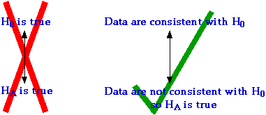
This distinction between the hypotheses is important. Depending on the sample data, it may be possible to conclude that HA is true. However, regardless of the data, the strongest we can say supporting H0 is that the data are consistent with it.
We can never conclude that H0 is likely to be true.
Memory test and exercise
Forty students in a psychology class are given a memory test. After a 30-minute session where the students undertake a variety of physical exercises, the students are given another similar memory test.
Has exercise has affected memory? The data are paired, so we analyse the difference in test results for each student ('after exercise' minus 'before exercise') and test whether the underlying population mean of these values is zero.
The diagram below illustrates the evidence obtained from a set of sample data.
Drag the slider to see the conclusions that might be reached for data sets with different means. The further the sample mean is from zero (on either side), the stronger the evidence that µ is not zero. We can get very strong evidence that H0 does not hold if the sample mean is far from zero.
However even ![]() = 0
does not provide strong evidence that µ = 0
= 0
does not provide strong evidence that µ = 0
If ![]() = 0,
µ
could just as easily be 0.0001 or -0.0002 (which correspond to HA).
We cannot distinguish, so the best we can say is that the data are consistent
with the null hypothesis — the data provide no information against the µ
being zero.
= 0,
µ
could just as easily be 0.0001 or -0.0002 (which correspond to HA).
We cannot distinguish, so the best we can say is that the data are consistent
with the null hypothesis — the data provide no information against the µ
being zero.
In the context of this example, the conclusion from a sample mean of zero would be that the experiment gave no evidence that exercise affected memory. Exercise might affect memory, but the experiment did not detect the effect.
The distinction between the null and alternative hypotheses is so important that we repeat it below.
We never try to 'prove' that H0 holds, though we may be able to 'prove' that HA holds.
Describing the credibility of the null hypothesis
In the previous page, a diagram with scales illustrated how the evidence against H0 was 'weighed' for different data sets. A p-value is a numerical description of this evidence that can give a scale to this diagram.
A p-value is a numerical summary statistic that describes the evidence against H0
Computer user-interface test
In an assessment of the user-interface of a computer program, sixteen users are shown a screen containing typical output for 10 seconds. Each user is then asked to indicate the position on the screen of a particular piece of information. The vertical distance between the indicated location and the actual location is recorded from each individual. (These 'errors' are negative if the user indicated too low a position.)
Do the users tend to pick the location of the item correctly, or is there a tendency to point too high or low? This question is equivalent to asking whether there is evidence that the underlying population mean of the 'errors' is different from zero.
The diagram below weighs the evidence using the p-value from a t-test of whether µ = 0.
The p-value is an index of credibility for the null hypothesis, µ = 0.
P-values have similar interpretation for all hypothesis tests.
Interpretation of p-values
Many different types of hypothesis test are commonly used in advanced statistics, but all share common features.
A p-value is a statistic that is evaluated from a random sample, so it has a distribution in the same way that a sample mean has a distribution. This distribution also has features that are common to all hypothesis tests. Understanding the distribution of p-values is the key to understanding how they are interpreted.
Distribution of p-values
In any hypothesis test,
The diagram below shows typical distributions that might be obtained.
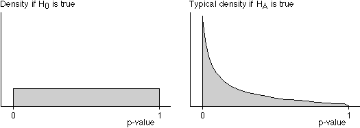
To illustrate these properties, we use a test for whether a population mean is zero.
In the diagram below, you will take random samples from a normal population for which H0 is true and, separately, from populations for which HA is true.
When H0 holds
Initially the population mean is zero, so H0 holds. A single sample from this population is shown on the left and the p-value for testing whether the population mean is zero is shown as a cross on the jittered dot plot on the bottom right.
Click the button Take sample a few times to take other samples from this population and add their p-values to the display on the bottom right. After taking 50 or more samples, you should observe that the p-values are spread evenly between 0 and 1. This supports our assertion that the p-values have a rectangular distribution between 0 and 1 when H0 holds.
When HA holds
Now use the slider to change the true population mean to 2.0. We are still testing whether the mean is zero, so HA now holds. Take 40 or 50 samples and observe that the p-values are usually closer to 0 than to 1.
Click on some of the larger p-values on the jittered dot plot to display the samples that gave rise to them. The sample means vary and, by chance, some samples have means that are near 0.0, even when the population mean is 2.0; these samples result in larger p-values.
Repeat this exercise with different population means (try at least 1.0, 2.0, 3.0 and -2.0). The further the population mean from the value targetted by H0, 0.0, the more tightly clustered the p-values are around 0.0.
Although it is possible to obtain a low p-value when H0 holds and a high p-value when HA holds, low p-values are more likely under HA than under H0.
P-values and probability
We saw in the last page that p-values have a rectangular distribution between 0 and 1 when H0 holds. A consequence of this is that the probability of obtaining a p-value of 0.1 or lower is exactly 0.1 (when H0 holds). This is illustrated on the left of the diagram below.
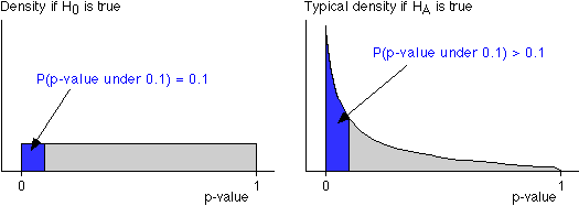
Similarly, the probability of obtaining a p-value of 0.01 or lower is exactly 0.01, etc. (when H0 holds).
| P-values are most likely to be near 0 if the alternative hypothesis holds |
Again, we use the specific hypothesis test for
in order to demonstrate these general results.
Click the button Take sample 50 or more times to take samples from this population and add their p-values to the display on the right. From the diagram on the top right, we can read off the proportion of p-values that are less than any value. Approximately 50% of p-values are less than 0.5, 20% are less than 0.2, etc. when the null hypothesis is true.
Use the slider to change the true population mean to 1.5 and repeat. From the diagram on the top right, you should observe that more than 50% of p-values are less than 0.5, more than 20% are less than 0.2, etc. when the alternative hypothesis holds.
Interpretation of p-value
Remembering that low p-values favour HA more than H0, we can give the following interpretation to a p-value.
If a data set gives rise to a p-value of say 0.0023, we can state that the probability of getting a data set with such a low p-value is only 0.0023 if H0 is true. Since such a low p-value is so unlikely, the data give strong evidence that H0 does not hold.
Of course, we may be wrong. A p-value of 0.0023 could arise when either H0 or HA holds. However it is unlikely when H0 is true and more likely when HA is true.
Similarly, p-value that is as low as 0.4 occurs with probability 0.4 when the null hypothesis holds. Since this is fairly high, we conclude from a data set that gave rise to a p-value of 0.4 that there is no evidence that the null hypothesis does not hold.
Although it may be regarded as an over-simplification, the table below may be used as a guide to interpreting p-values.
| p-value | Interpretation |
|---|---|
| over 0.1 | no evidence that the null hypothesis does not hold |
| between 0.05 and 0.1 | very weak evidence that the null hypothesis does not hold |
| between 0.01 and 0.05 | moderately strong evidence that the null hypothesis does not hold |
| under 0.01 | strong evidence that the null hypothesis does not hold |
Applying the general properties of p-values to different tests
The properties of p-values (and hence their interpretation) have been demonstrated in the context of a hypothesis test about whether a population mean was zero.
P-values for all hypothesis tests have the same properties. As a result, we can interpret any p-value if we know the null and alternative hypotheses that it tests, even if we do not know the formulae that underlies it. (In practice, a statistical computer program is generally used to perform hypothesis tests, so knowledge of formulae is of little importance.)
In particular, for any test where the null hypothesis restricts a parameter to a single value,
| p-value | Interpretation |
|---|---|
| over 0.1 | no evidence that the null hypothesis does not hold |
| between 0.05 and 0.1 | very weak evidence that the null hypothesis does not hold |
| between 0.01 and 0.05 | moderately strong evidence that the null hypothesis does not hold |
| under 0.01 | strong evidence that the null hypothesis does not hold |
Another type of test
The normal distribution is often used as a hypothetical population from which a set of data are assumed to be sampled. But are the data consistent with an underlying normal population, or does the population distribution have a different shape?
One popular test for assessing whether a random sample come from a normal population is the Shapiro-Wilkes W test. The theory behind the test is advanced and the formula for the p-value cannot be readily evaluated by hand. However most statistical programs will perform the test.
A random sample of 40 values from a normal population is displayed in a jittered dot plot on the left of the diagram. The p-value for the Shapiro-Wilkes W test is shown under the dot plot and also graphically on the right.
Click Take sample a few times to take more samples and build the distribution of the p-values for the test. You should observe that the p-values have a rectangular distribution between 0 and 1 when the null hypothesis is true (i.e. if the samples are from a normal distribution).
Drag the slider on the top left of the diagram to change the shape of the population distribution. Repeat the exercise above and observe that when the null hypothesis does not hold, the p-values tend to be closer to 0.
Click on crosses on the display of p-values in the bottom right to display the sample that produced that p-value. P-values near zero usually correspond to samples that have very long tails to one or both sides, or have very short tails to one or both sides.
Measuring the speed of light
As a numerical example, consider the following experimental measurements made by a scientist, Simon Newcomb, in 1882 for the purpose of estimating the speed of light in air. The values were the times in nanoseconds (0.000000001 seconds) for light to travel 7442 metres. Since the measurements were all close to 24,800, they have been coded
| Raw data (nanoseconds) | Coded data |
|---|---|
| 24,828 | 24,828 - 24,800 = 28 |
| 24,826 | 24,826 - 24,800 = 26 |
| etc | etc |
The coded data and a histogram are shown below.
| 28 26 33 24 34 -44 27 16 40 -2 29 22 24 21 25 30 23 29 31 19 24 20 36 32 36 28 25 21 28 29 37 25 28 26 30 32 36 26 30 22 36 23 27 27 28 27 31 27 26 33 26 32 32 24 39 28 24 25 32 25 29 27 28 29 16 23 |
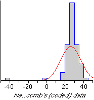 |
The best-fitting normal distribution (with mean and standard deviation equal to those of the data) has been superimposed on the histogram. Could the two 'outliers' in the data have occurred by chance from a normal population?
Applying the Shapiro-Wilkes W test to the data using the statistical program JMP gives a p-value '0.0000'. Since JMP rounds p-values to four decimal places, this really means that the p-value is less than 0.00005. We therefore conclude that the probability of obtaining such a non-normal looking sample from a normal distribution is less than 0.00005, so there is extremely strong evidence that the data do not come from a normal population.
In contrast, if the two 'outliers' are omitted, JMP reports a p-value of 0.6167 for the test. Since a p-value as low as this would be found from 62% of samples from a normal population, there is no evidence that the data without the outliers are non-normal. The test therefore lends support to the assertion that the two outliers resulted from errors in Newcomb's experimental procedures.
You should be able to interpret p-values that computer software provides for a wide variety of hypothesis tests using the properties that we have described in this section.